
Open the model
Worked example: Warkworth
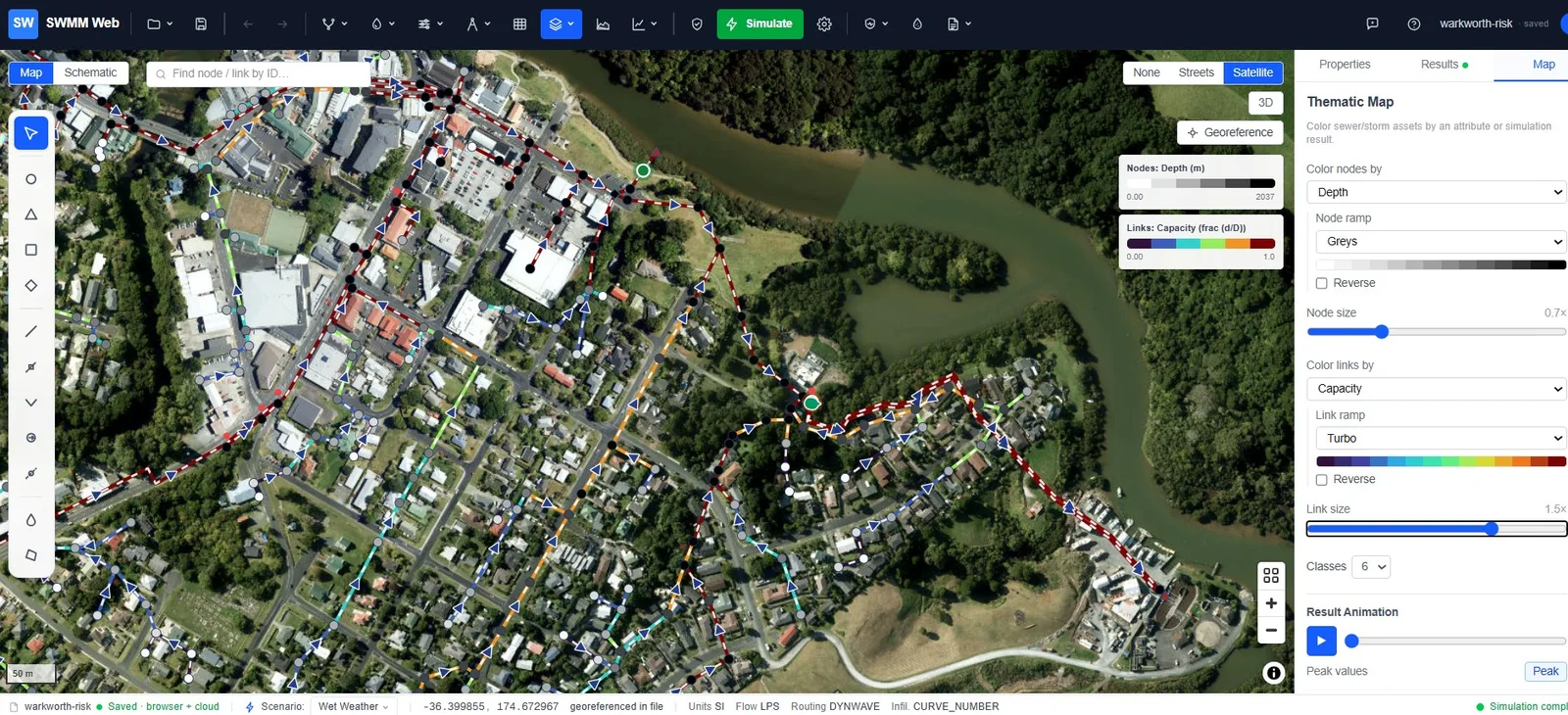
Warkworth, north of Auckland, is a combined sewer of 873 junctions and 875 conduits serving a town that drains to a treatment plant through two pumping stations. When a large storm arrives, an overflow structure spills the excess to a stream rather than backing it up into streets and houses.
That makes it the example to follow once Watertown has shown you the basics. Watertown teaches the interface; Warkworth asks the harder question - is the model right? - and gives you a day of measurements to answer it with.
Download the files
warkworth.inp · warkworth-scada.csv · warkworth-live.inp (Live Ops / SCADA demo) · warkworth-idf.csv · warkworth-risk.inp · warkworth-condition-sample.csv
What is in the model
Section titled “What is in the model”| Network | 873 junctions, 875 conduits, combined system |
| Pumping | WRPS and LSPS, two duty pumps each, drawing from a wet well |
| Storage | Two wet wells - WRPS_WW (1.95 m deep) and LSPS_WW (2.40 m) |
| Discharge | WWTP - the treatment plant |
| Overflow | Overflow - the CSO, spilling from manhole MH-6801 |
| Event | A 10-year design storm over 24 hours, 3-minute reporting |
| Control | Eight rules starting and stopping pumps on wet-well level |
The goal
Section titled “The goal”A model is only worth acting on if it reproduces something that actually happened. Warkworth ships with the observed record for the same day, so you can put three questions to it in order:
-
Did it conserve water? Continuity first - nothing downstream matters if it failed.
-
Do the wet wells fill and empty like the real ones? This tests the pumps and the control rules.
-
Does the CSO spill the right amount, at the right time? This is the question a regulator asks, and the one an operator needs answered before the storm, not after.
Modelling notes
Section titled “Modelling notes”Dynamic-wave routing. A network with pumps switching against wet wells cannot be routed
kinematically - the backwater and the storage matter. Open Calculation options and you
will find the settings that make it stable: INERTIAL_DAMPING PARTIAL, VARIABLE_STEP 0.75
and LENGTHENING_STEP 10.
Pump control in one place. SWMM lets you set pump start and stop levels twice - as startup
and shutoff depths on the pump itself, and as rules in [CONTROLS]. Both act. In this model
they originally disagreed, so the pumps started half a metre early and the wet well never
reached its real level. The model ships with rules as the single source of truth, and the
pump depths cleared. If a pump behaves oddly, check whether it is being told two things.
Checking against SCADA
Section titled “Checking against SCADA”The observed record is a 24-hour, 3-minute file covering the storm. Open
Model data ▸ Monitoring data (SCADA)…, load warkworth-scada.csv, and each sensor column
appears as a row to be mapped to a model element. Once imported, the measurements overlay as
a dashed line on the Results chart of whichever element you select.
Which signal goes where
Section titled “Which signal goes where”Fill the dialog’s Element, ID and Variable columns like this:
| Sensor column | Element | ID | Variable | What it is |
|---|---|---|---|---|
Overflow | Link | Overflow | Flow | The CSO spill - the headline number |
LSPS_Inflow | Link | 29512564 | Flow | Trunk main arriving at the LSPS wet well |
WRPS_Outflow | Link | P-15 | Flow | Rising main carrying both WRPS pumps |
WRPS_WW_Depth | Node | WRPS_WW | Depth | Wet-well level at WRPS |
LSPS_WW_Depth | Node | LSPS_WW | Depth | Wet-well level at LSPS |
The two wet wells are storage nodes, so their signal is a depth. Everything else is a
flow through a link. Overflow is both a conduit and the outfall it discharges to - map
the sensor to the conduit, which is where the spill rate is carried.
What you should see
Section titled “What you should see”| Observed | Simulated | |
|---|---|---|
| CSO spill volume | 107 m³ | 106 m³ |
| CSO onset | 11:57 | 11:57 |
| CSO peak | 19.4 L/s | 14.6 L/s |
| LSPS wet-well level | correlation 0.78 | |
| LSPS trunk inflow | correlation 0.95 |
Spill volume and timing both land. The peak does not - the model spreads the same water over a flatter hydrograph, under-predicting the instantaneous rate by about a quarter.
Climate resilience
Section titled “Climate resilience”The interesting question is not what this storm did. It is what a bigger one would do.
-
Establish the baseline. Run as shipped and note the spill volume - about 106 m³ from a 10-year event.
-
Open the tool. Toolbar → Resilience & adaptation (the shield icon) → Flood & climate resilience…. This is a Pro feature; on the free plan the menu item opens the upgrade dialog instead.
-
Load the site rainfall. In the Site rainfall statistics (IDF / DDF) panel press Import CSV… and choose warkworth-idf.csv. The curves plot on log-log axes, one per return period. Pick a return period, set a duration - or click the chart - and press Use this depth → to send it to the storm builder. Without a file the panel falls back to a regional preset, clearly marked as indicative rather than site data.
-
Find where it breaks. Re-run each and record the spill volume. A system with real headroom shows a long flat stretch then a sharp rise; a stressed one starts spilling almost immediately.
-
Add climate uplift. Apply a rainfall-intensity uplift to the design storm - the dialog offers Present-day, Mid-century (+2 °C, about +15%) and End-century (+4 °C, about +30%) - then re-run. A 20-year system under 30% more rain is not a 20-year system any more, and putting a number on that shift is what a resilience case is made of.
-
Test an intervention. Add storage upstream of the overflow, or change the pump rules to draw the wet wells down ahead of the peak, and re-run. The difference in spill volume is the benefit, in the units a regulator counts.
From risk to a capital plan
Section titled “From risk to a capital plan”The same model that reproduces the spill can also decide which pipes to renew and in what order. Open the register from Resilience & adaptation ▸ Asset risk register (CIP) (a Utility-tier feature). It scores every conduit as Risk = Probability × Consequence of failure, where consequence is read from the hydraulics you already ran - how much of the network drains through a pipe, the sewershed it serves, whether its failure reaches the CSO or outfall - not a hand-entered field. Run the simulation first so the probability score includes hydraulic stress.
-
Read the register. A 5×5 heatmap and a ranked table; the map shades every conduit by risk band. Click a pipe to see a what-if: reline / replace / upsize / defer, each with an estimated cost, the resulting risk and the value (risk reduction per dollar).
-
Add condition data. Real risk needs real condition. Use Import condition data with warkworth-condition-sample.csv (a small starter set keyed to conduit IDs), or your own CCTV survey as a CSV or a shapefile attribute table. Pick the coding standard - PACP (US), MSCC (UK) or EN 13508 (EU) - and SWMM Web normalises the grade; a survey grade overrides the age estimate. See Sewer condition grading.
-
Optimise the programme. Open Capital plan (CIP), set an annual budget (or “fund-all”), and Optimise. It funds the best risk-reduction-per-dollar option on each pipe within budget and reports how far the risk comes down and how many high-risk pipes are still unfunded. Export a CIP PDF for the board pack.
-
Verify, don’t promise. Click Apply to model - upsizes become real larger diameters, reline/replace record as-new condition - then re-run. The register drops because the pipes now run less full and are in better condition. That closing loop, consequence you can simulate, is what a spreadsheet-based risk score cannot do.
-
Fund it. Open Financial plan (20-yr) to turn the programme into a payment plan. Enter the utility’s rate revenue, O&M and reserves (US SRF + bond defaults are pre-filled), and the solver phases the work across 20 years, splits it into debt and PAYGO, and finds the steady rate increase that funds it while holding debt-service coverage and days-cash above target. Export a financing PDF for the board. See Financial plan (debt / PAYGO).
For the full method see Asset risk register. The warkworth-risk.inp model above is a ready copy to run this on.
Worked example: funding the Warkworth programme
Section titled “Worked example: funding the Warkworth programme”Run the four steps on warkworth-risk.inp with the sample condition data and you get a real
programme, not a slogan. The register scores all 875 conduits (260 very-high, 407 high), and
“fund-all” builds a $4.9M renewal programme - 800 pipes, mostly relining with a handful of
upsizes where hydraulics, not condition, drive the risk.
Open Financial plan (20-yr) and it seeds a small-utility profile from the programme size (~$705k annual rate revenue, ~$388k O&M) - every field editable. The solver returns:
+1.5% / year
The steady rate increase that funds the whole programme. No spike.
50 / 50 debt / PAYGO
Half from cheap SRF and bond debt (matched to the assets’ long life), half cash from rates.
1.32x minimum DSCR
Debt-service coverage never drops below target across the 20 years; 291 days cash in hand throughout.
~$640k interest
The total cost of borrowing over the term - the price of spreading it fairly across future users.
For Warkworth that programme is comfortably affordable: the whole $4.9M funds at any rate ceiling from 2%/yr up. The trade-off the tool is really built for shows when money is tight. Give it a smaller utility (say $500k revenue, $400k O&M) and the affordability-vs-risk curve slopes:
| Max rate increase | Programme funded | High-risk pipes still unfunded |
|---|---|---|
| +2.0% / yr | $0.4M | 616 |
| +2.5% / yr | $1.9M | 392 |
| +3.0% / yr | $3.0M | 207 |
| +3.5% / yr | $4.0M | 49 |
| +4.0% / yr | $4.9M (all) | 0 |
That is a rate case grounded in hydraulics: at 2%/yr you leave 616 high and very-high pipes in the ground; step to 4%/yr and you clear them all. This same utility funds the full programme at +3.9%/yr (74/26 debt/PAYGO), inside a normal affordability band - a spreadsheet cannot connect the rate you can pass to the flooding risk you retire.
What this example does not show
Section titled “What this example does not show”Being clear about the edges is part of the example:
- Peak spill rate is under-predicted by about 25%. Volume and timing are calibrated; the instantaneous peak is not.
- The pump flow record stops before the storm begins, so pump discharge is validated only against the dry days preceding the event - not against the storm itself.
- The WRPS wet well matches on average but not in shape. Its pumps cycle faster than the 3-minute sampling interval resolves, so the record cannot see individual cycles.
- Reading results - what continuity, surcharge and flooding actually mean
- CSO forecasting - driving this model from a weather forecast
- Design storms and climate uplift - building the events used above