
Flex Tables
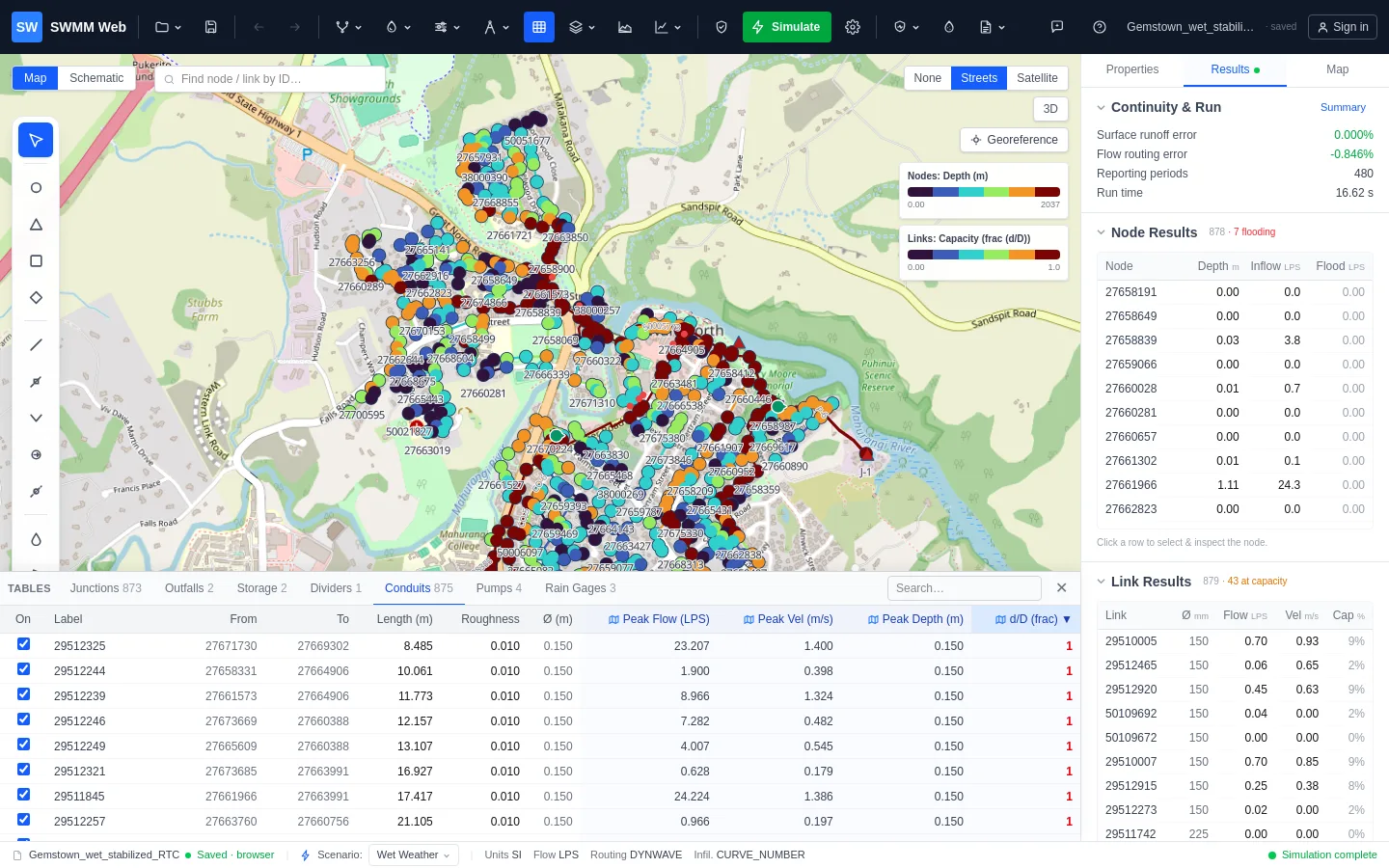
Flex Tables dock along the bottom of the window: a tabbed grid with one tab per element type, showing every junction, conduit, subcatchment and the rest. It is the fastest way to work with a network as data rather than as a picture.
What you can do in it
Section titled “What you can do in it”Sort by any column. Click a header. Click again to reverse. Sorting the conduits by d/D
descending puts the most surcharged pipe in the network on the first row, which is usually
where an investigation should start.
Search. Narrow to the elements whose id matches, when you know roughly what you are looking for.
Edit in place. Double-click a cell. Input properties are editable here exactly as they are in the Properties panel, and edits are undoable in the same way.
Jump to the map. Click a row to select that element and fly the map to it. On a large network this is far quicker than hunting visually.
Shade the map from a column. Result columns carry a small map button that sets the thematic styling to that attribute, so you can go from a sorted table to a shaded map in one click.
Active topology
Section titled “Active topology”Each row carries a checkbox. Unchecking an element excludes it from the run without deleting it.
This is how you test a network without destroying it: take a relief sewer out and re-run to see the pre-scheme condition, switch off a pump to see what happens when it fails, or isolate a branch you suspect is mis-connected. The element stays in the model with all its properties intact, and the checkbox is the only thing that changed.
Active topology is stored per scenario, so a scheme scenario can have a different set of elements enabled from the baseline, and switching scenarios switches the topology with it. See scenarios.
Getting the data out
Section titled “Getting the data out”The table is the same data the CSV exports produce, so anything you can sort and read here can leave as a file from the Results panel. For plotting a series through time rather than reading peaks, use the graph.