
Reading the results
A run produces a value for every element at every time step. The skill is not reading it all, it is knowing what to look at.
Start with the tables
Section titled “Start with the tables”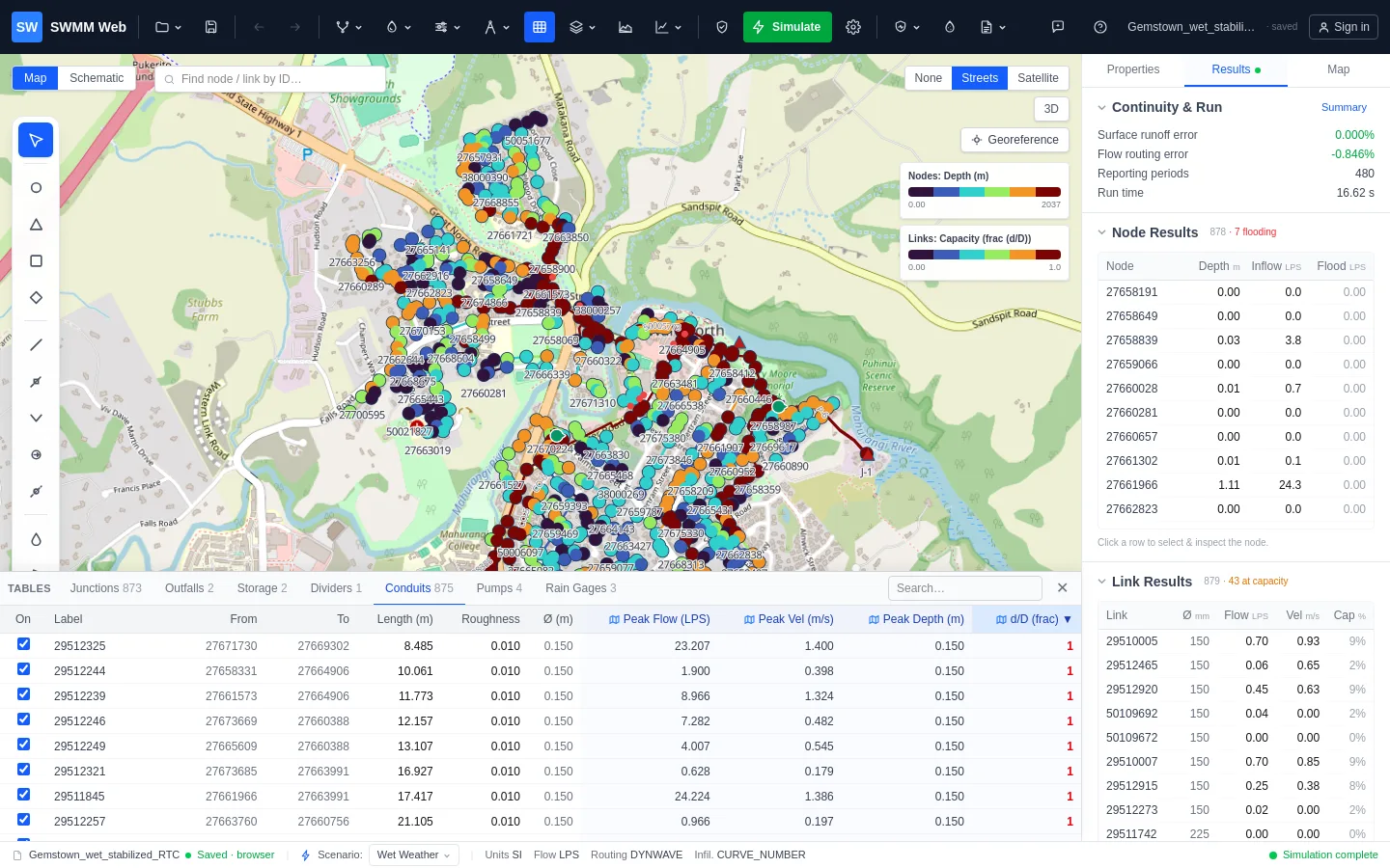
Open Flex Tables. After a run, result columns appear beside the model properties:
Nodes: peak depth, head, inflow, flooding, and freeboard - the spare depth between the peak water level and the rim. Negative freeboard means the node surcharged above ground.
Links: peak flow, velocity, depth, and d/D - how full the pipe ran, where 1.0
is completely full.
Result columns are read-only, because they are outputs. They turn red at the thresholds
that mean failure: d/D at or above 1, any flooding, freeboard at or below zero.
Then look at where
Section titled “Then look at where”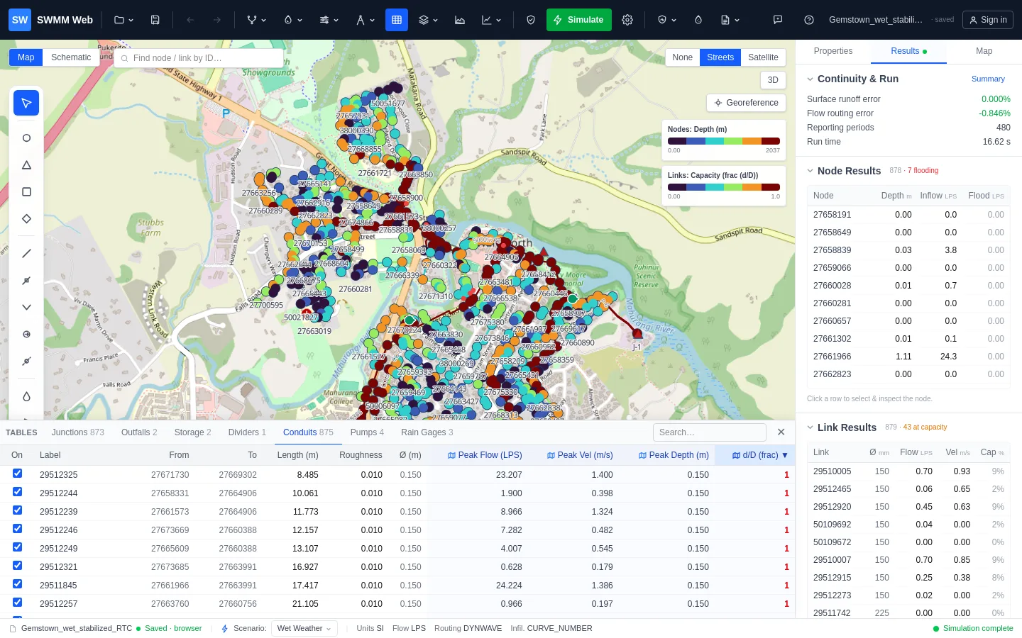
A list tells you how many. A map tells you where, and the spatial pattern is what distinguishes two very different problems.
Click the small map icon in any result column header, or use the Map panel to colour
nodes and links by any attribute. Shading by d/D:
- One continuous red run - a single real bottleneck. Fix that reach and everything upstream improves.
- Scattered red spots - usually not capacity at all, but local slope or invert-offset errors. Resizing those pipes would treat a symptom.
Head loss along a conduit
Section titled “Head loss along a conduit”The Conduits table carries a Head loss column, and the map can be shaded by head loss, so the pipes actually costing you head stand out without reading a table.
SWMM saves a head per node and a velocity per link, but never a loss per link, so this is derived - and derived the way the engine derives it, from the same constants, so the number agrees with what the solver did rather than merely resembling it:
head loss = S_f · L + (Kentry + Kexit + Kavg) · V² / 2gFriction comes from Manning, S_f = (n / 1.486)² · V² / R^(4/3), mirroring link.c. A
force main flowing full does not use Manning at all, and the Hazen-Williams or
Darcy-Weisbach form is used instead, following the model’s own FORCE_MAIN_EQUATION setting.
Profiles
Section titled “Profiles”The Profile tool draws a longitudinal section along a path: ground level, pipe inverts, and the hydraulic grade line. This is where surcharge becomes obvious - you see the water level climb above the pipe crown and how far up the manhole it goes.
Pick an upstream and a downstream node and the path between them is found automatically.
Graphs
Section titled “Graphs”Quick graph puts a time series on screen for whatever you click. Graph details gives the full interactive chart: multiple series, a second Y axis, zoom, export to PNG or CSV, and saved presets.
Overlaying an observed SCADA series on a modelled one is how you judge whether a model is believable. See the calibration guides.
Animation
Section titled “Animation”In the Map panel, step or play through reporting periods. The colour scale stays fixed at the peak distribution so the legend does not move under you - only the elements change.
Watching a storm pass through the network shows you the order things fail in, which a peak value cannot.
Exporting
Section titled “Exporting”Node and link summaries as CSV, the full time series as CSV, the SWMM .rpt, and a
printable report that includes the design check and its suggested next steps.