
Watertown, metric
Open the demo → - 327 junctions, LPS / hectares / mm.
This guide takes you from nothing to a model you have built, run and read the results of. It takes about fifteen minutes. You do not need to install anything, and you do not need an account.
Go to app.swmmweb.com. That is the whole installation step.
SWMM Web runs the real EPA SWMM 5.2 engine, inside your browser. Your model is not uploaded anywhere to be simulated - the solver executes on your own machine. This matters if your network data is confidential, and it is why the application keeps working when your connection does not. See Local-first, offline and your data.
If you would rather start from something that already exists, you can open your own
.inp file, or load a demo:
Watertown, metric
Open the demo → - 327 junctions, LPS / hectares / mm.
Watertown, US units
Open the demo → - the same network in CFS / acres / inches.
This is the fastest route to a working model, and the one worth trying first.
In the toolbar, choose Project ▸ Generate model from location.
Type a place name - a town, a street, a postcode - and press Enter. The map moves there.
Choose the study area. Drag the rectangle, or switch to polygon mode and trace the real service area. Tracing a polygon is worth the extra few seconds: everything inside it is treated as draining to the network, so a rectangle that includes a hillside or a lake will inflate the runoff.
Pick the system type:
Press Generate.
What happens next is worth understanding, because it explains the numbers you are about to see. The application pulls the street layout from open source datasets, samples ground elevation from a world terrain dataset, lays manholes at junctions and pipes along the streets, routes everything downhill to an outfall, and sizes each pipe from the catchment draining to it.
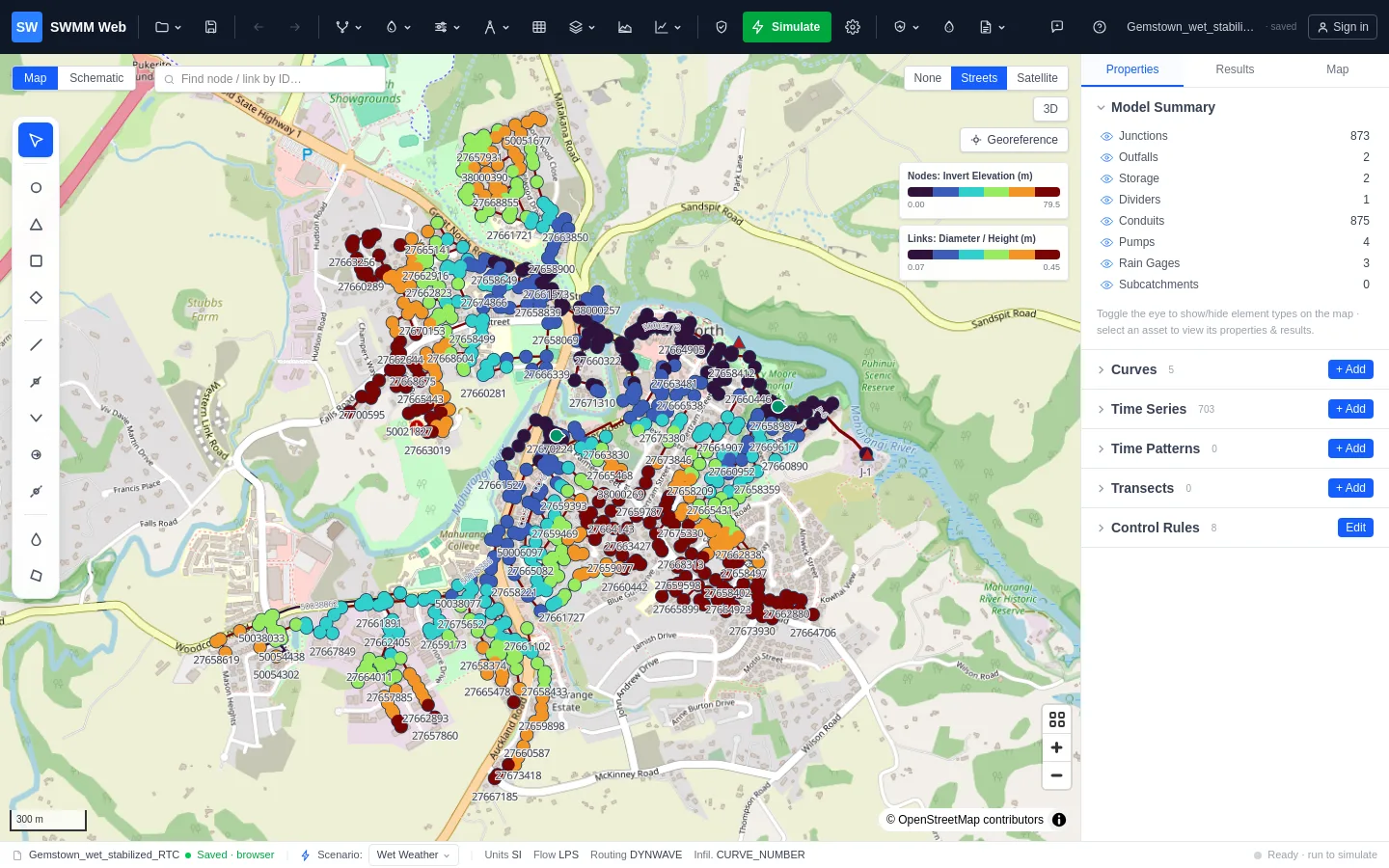
Four regions, and you will use all of them.
| Region | What it is for |
|---|---|
| Toolbar (top) | Files, drawing tools, simulation, results, reporting, operational data |
| Map (centre) | The network. Click any element to select it; drag to move it |
| Panels (right) | Properties of what you selected, and map styling |
| Status bar (bottom) | Units, scenario, and the state of the current run |
Two panels are worth opening straight away:
Press Simulate in the toolbar.
Wait. A small network takes a second or two; a few hundred nodes with dynamic-wave routing takes longer, because it is solving the real hydraulics.
The summary appears automatically when it finishes: run time, continuity error, how many nodes flooded, and any warnings the engine raised.
This is the step people skip, and it is where the value is.
Open Flex Tables, choose the Conduits tab, and click the d/D column header
twice to sort descending. d/D is how full each pipe ran: 1.0 means completely full.
The pipes at the top of that list are your bottlenecks, and anything at or above 1.0
is shown in red.
Click any row and the map flies to that pipe.
In the Results tab, open Design check. It reads the whole run and returns a ranked list of what is wrong - flooding, surcharge, pipes at capacity, velocities below self-cleansing, adverse slopes - each with a locate → link, plus suggested next steps ordered by what matters first.
That ordering is deliberate: fix connectivity before slope, and slope before sizing. A model that cannot drain is not worth resizing.
A list of 152 full pipes tells you how many. Press Shade map by d/D and you see where - and the pattern tells you which problem you have:
Press Save (the icon beside the Project menu) to keep the project in this browser. To get
a file, choose Project ▸ Export SWMM model (.inp): it is written to your own computer as a
standard SWMM .inp - the same format EPA SWMM, PCSWMM and InfoSWMM read. Nothing is
locked in.
If you sign in, you can also save models to the cloud (one on the Free plan, unlimited on Pro) and, on Pro, share them with colleagues, but that is optional. The application works without an account.